Recent advances on VI
Contents
Recent advances on VI
For a survey of recent advances in Variational Inference, I highly recommend Zhang et al 2018. Some of the topics presented in this survey are discussed here
Recap from previous lectures
We are interested in a posterior
which may be intractable. If that is the case we do approximate inference either through sampling (MCMC) or optimization (VI).
In the latter we select a (simple) approximate posterior \(q_\nu(\theta)\) and we optimize the parameters \(\nu\) by maximizing the evidence lower bound (ELBO)
which makes \(q_\nu(\theta)\) close to \(p(\theta|\mathcal{D})\)
Note
There is a trade-off between how flexible/expressive the posterior is and how simple is to approximate this expression
In what follows we review different ways to improve VI
More flexible approximate posteriors for VI
Normalizing flows
One way to obtain a more flexible and still tractable posterior is to start with a simple distribution and apply a sequence of invertible transformations. This is the key idea behind normalizing flows.
Let’s say that \(z\sim q(z)\) where \(q\) is simple, e.g. standard gaussian, and that there is a smooth and invertible transformation \(f\) such that \(f^{-1}(f(z)) = z\)
Then \(z' = f(z)\) is a random variable too but its distribution is
which is the original distribution times the inverse of jacobian of the transformation
And we can apply a chain of transformations \(f_1, f_2, \ldots, f_K\) obtaining
With this we can go from a simple Gaussian to more expressive/complex/multi-modal distributions
Nowadays several types of flows exist in the literature, e.g. planar, radial, autoregresive. As example, see this work in which normalizing flows were used to make the approximate posterior in VAE more expressive
Key references:
Dinh, Krueger and Bengio, “NICE: Non-linear Independent Components Estimation”
Rezende and Mohamed, “Variational Inference with Normalizing Flows”
Kingma and Dhariwal, “Glow: Generative Flow with Invertible 1x1 Convolutions”
Adding more structure
Another way to improve the variational approximation is to include auxiliary variables. For example in Auxiliary Deep Generative Models the VAE was extended by introducing a variable \(a\) that does not modify the generative process but makes the approximate posterior more expressive
In this case the graphical model of the approximate posterior is \(q(a, z |x) = q(z|a,x)q(a|x)\), so that the marginal \(q(z|x)\) can fit more complicated posteriors. The graphical model of the generative process is \(p(a,x,z) = p(a|x,z)p(x,z)\), i.e. under margnalization of \(a\), \(p(x,z)\) is recovered
The ELBO in this case is
Tigher bounds for the KL divergence
Importance weighting
This is an idea based on importance sampling. Tigher bounds for the ELBO can be obtained by sampling several \(z\) for a given \(x\). This was explored for autoencoders in Importance Weighted Autoencoders
Let’s say we sample independently \(K\) times from the posterior, this yields progressively tighter lower bounds for the evidence:
where \(w_k = \frac{p_\theta(x, z_k)}{q_\phi(z_k|x)}\) are called the importance weights. Note that for \(K=1\) we recover the VAE bound.
This tighter bound has been shown to be equivalent to using the regular bound with a more complex posterior. Recent discussion can be find in Debiasing Evidence Approximations: On Importance-weighted Autoencoders and Jackknife Variational Inference and Tighter Variational Bounds are Not Necessarily Better.
Other divergence measures
\(\alpha\) divergence
The KL divergence is computationally-convenient but there are other options to measure how far two distributions are. For example the family of \(\alpha\) divergences (Renyi’s formulation) is defined as
where \(\alpha\) represents a trade-of between the mass-covering and zero-forcing effects. The KL corresponds to the special case \(\alpha \to 1\)
Note
The \(\alpha\) divergence has been explored for VI recently and is implemented in numpyro
f divergence
The \(\alpha\) divergence is a particular case of the f-divergence
where \(f\) is a convex function with \(f(0) = 1\). The KL is recovered for \(f(z) = z \log(z)\)
In general \(f\) should defined such that the result in the bound does not depend on the marginal likelihood. Wang, Liu and Liu, 2018 proposed tail-adaptive f-divergence
Stein variational gradient descent (SVGD)
Another totally different approach is based on the Stein operator
where \(p(x)\) is a distribution and \(\phi(x) = [\phi_1(x), \phi_2(x), \ldots, \phi_d(x)]\) a smooth vector function
Under this following, known as the Stein identity, holds
Now, for another distribution \(q(x)\) with the same support as \(p\), we can write
from which the Stein discrepancy between two distributions is defined
Which to actually work requires \(\mathcal{F}\) to be broad enough
This is were kernels can be used. By taking an infinite amount of basis function \(\phi(x)\) on the stein discrepancy it can be shown that the optimization is solved by
where \(\kappa\) is a kernel function, e.g. RBF or rational quadratic. From this one can use stochastic gradient descent.
See also
For a more in depth treatment see this list of papers related to SVGD
Operator VI
Ranganath et al. 2016 proposed to replace the KL divergence as objective for VI with the Langevin-stein operator
