Linear Latent Variable Models
Contents
Linear Latent Variable Models
Modeling with latent variables
Let’s say we have a dataset \(X = \{ \textbf{x}_1, \textbf{x}_2, \ldots, \textbf{x}_N\}\) with \(\dim (\textbf{x}) =D\) and we want to model the generative distribution \(p(\textbf{x})\)
Each sample has \(D\) components or attributes (e.g. the pixels of an image): These are the observed variables
To model \(p(\textbf{x})\) we may expand the joint probability between the attributes using the rules of probability
which is known as a fully observed model
Warning
Unless we introduce independence between some of the variables the above representation is impractical for high dimensional problems (e.g. images)
Hint
Assume that what we observe is correlated due to hidden causes
These hidden causes are represented as latent variables and models with latent variables are called Latent Variable Models (LVMs)
Mathematically, we impose that the observed variables are conditionally independent given the latent variables \(\textbf{z}\), this is
where in general \(\dim(\textbf{z})\ll\dim(\textbf{x})\)
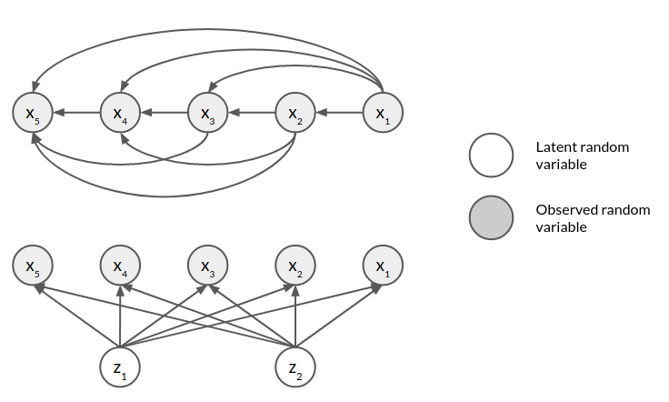
The following figure shows the graphical model of a fully observed model with five observed variables and an LVM with two latent variables
For the LVM we can write the marginal as
Did we gain anything? (YES)
Important
This strategy allows us to model a complex \(p(x)\) by proposing a simple \(p(z)\) (easy to sample from) and a transformation \(p(x|z)\)
The integral above is intractable for non-linear transformations (neural networks), in that case we resort to approximate inference
This lecture is focused on LVMs for continuous data. First we will review an example with a tractable posterior (PCA) and then the more modern LVM based on neural networks: The Variational Autoencoder
A short review of PCA
Principal Component Analysis (PCA) is an algorithm to reduce the dimensionality of continous data
For a dataset \(X = (x_1, x_2, \ldots, x_N) \in \mathbb{R}^{N \times D}\), in PCA we
Compute covariance matrix \(C = \frac{1}{N} X^T X\)
Solve the eigenvalue problem \((C - \lambda I)W = 0\)
This comes from the following objective
i.e. PCA finds an orthogonal transformation \(W\) that maximizes the variance of the projected data \(XW\)
Important
By reducing the amount of columns of \(W\) we reduce the dimensionality of \(XW\)
Example: Classical PCA for MNIST using JAX
We will use the MNIST handwritten digits dataset:
import os
import sys
sys.path.append(os.path.abspath(os.path.join('../utils')))
from mnist import mnist
train_images, train_labels, test_images, test_labels = mnist()
import holoviews as hv
hv.extension('bokeh')
hv.opts.defaults(hv.opts.Image(cmap='gray', xaxis=None, yaxis=None))

examples = [hv.Image(example.reshape(28, 28)) for example in test_images[:10]]
hv.Layout(examples).opts(hv.opts.Image(width=100, height=100)).cols(5)


Implementation of PCA using jax.numpy.eigh:
import numpy as np
import jax.numpy as jnp

class PCA:
    def __init__(self, data, K=2):
        self.data_mean = data.mean(axis=0)
        data_centered = data - self.data_mean
        C = jnp.dot(data_centered.T, data_centered)
        L, W = jnp.linalg.eigh(C, symmetrize_input=False)
        # eigh, returns sorted by L (eigenvals) in ascending order
        self.L = L[-K:]
        self.W = W[:, -K:]

    def get_eigenvalues(self):
        return self.L

    def encode(self, x):
        return jnp.dot(x - self.data_mean, self.W)

    def decode(self, z):
        return self.data_mean + jnp.dot(z, self.W.T)
In this example the \(28\times28\) observed dimensions of PCA are projected to two continuous latent variables
pca = PCA(train_images, K=2)
z = pca.encode(test_images)
xhat = pca.decode(z)
z
WARNING:absl:No GPU/TPU found, falling back to CPU. (Set TF_CPP_MIN_LOG_LEVEL=0 and rerun for more info.)
DeviceArray([[-2.9325423 ,  1.3030709 ],
             [ 3.747396  , -0.08111978],
             [ 1.6895869 ,  3.7099552 ],
             ...,
             [-2.3406672 ,  1.0596066 ],
             [ 0.42589757,  1.2315243 ],
             [ 0.35495937, -4.087756  ]], dtype=float32)
We can then inspect the latent space and images reconstructed from it
scatter_plot = []
for digit in range(10):
    mask = test_labels.argmax(axis=1) == digit
    scatter_plot.append(hv.Scatter((z[mask, 0], z[mask, 1]), 'z0', 'z1', label=f"{digit}"))

hv.Overlay(scatter_plot).opts(width=550, height=400, legend_position='right')
examples = [hv.Image(example.reshape(28, 28)) for example in test_images[:5]]
reconstructed = [hv.Image(example.reshape(28, 28)) for example in np.array(xhat[:5])]

hv.Layout(examples + reconstructed).opts(hv.opts.Image(width=100, height=100)).cols(5)
The two most important principal components in this case are
eigvectors = [hv.Image(np.array(eigvec.reshape(28, 28))) for eigvec in pca.W.T]
hv.Layout(eigvectors).opts(hv.opts.Image(width=200, height=200))
Note
Clearly wwo continous latent variables are not enough to model the digits given this linear model. Later we will see how this changes using non-linear models
Probabilistic interpretation for PCA
We can give a probabilistic interpretation to PCA as an LVM
The observed data \(x_i \in \mathbb{R}^D\) is modeled as
where
\(B \in \mathbb{R}^D\) is the mean of \(X\)
\(W \in \mathbb{R}^{D\times K}\) is a linear transformation matrix
\(\epsilon\) is a noise vector
\(z_i \in \mathbb{R}^K\) is a continuous latent variable with \(K\ll D\)
Note
\(x\) (observed) is related to \(z\) (latent) via a linear mapping
The PCA model has the following assumptions
The noise is independent and Gaussian distributed with variance \(\sigma^2\)
The latent variable has a standard Gaussian prior
Using these we can write
and
Given that the Gaussian is conjugate to itself the marginal likelihood is
Note
We have parameterized a Gaussian with full covariance from two Gaussians with diagonal covariance
::
The parameters of the marginal come from
\(\mathbb{E}[x] = W\mathbb{E}[z] + B + \mathbb{E}[\epsilon] = B\)
\(\mathbb{E}[(Wz + \epsilon)(Wz + \epsilon)^T] = W \mathbb{E}[zz^T] W^T + \mathbb{E}[\epsilon \epsilon^T] = W W^T + I\sigma^2\)
The posterior
Using this formalism we can write the posterior as
which can be used to move from observed to latent dimension, where
Training
We find \(W\), \(B\) and \(\sigma\) that best fit the data by maximizing the log marginal likelihood
which has a closed form analytical solution.
Note
The solution for \(W\) is equivalent to conventional PCA (\(\sigma^2 \to 0\)). The main difference is that we have \(\sigma\) and we can generate data with \(p(x|z)p(z)\)
See also
For more details on PCA and probabilistic PCA see chapters 15 and 21 in D. Barber’s book