Stochastic Variational Inference with NumPyro
Contents
Stochastic Variational Inference with NumPyro
Previously we learned
how to write probabilistic models and perform MCMC with
numpyrothe fundamental ideas of variational inference (VI)
In this lesson we will explore the tools offered by numpyro to obtain approximate variational posteriors. The unified interface for VI in numpyro is located in numpyro.infer.SVI
The arguments of the SVI object are
numpyro.infer.SVI(model, # A function that defines the generative model
                  guide, # A function that defines the approximate posterior
                  optim, # A "gradient-descent-based" optimizer
                  loss, # The cost function, a variant of the ELBO
                  static_kwargs # (Optional) Static arguments of model
                 )
See also
SVI corresponds to Stochastic Variational inference, a methodology to scale VI to large databases by subsampling. In SVI, the cost function and its derivatives are estimated as averages over minibatches of data. In summary, SVI is the combination of VI and Stochastic Gradient Descent (SGD)
Through this lesson we consider the following data as example
import holoviews as hv
hv.extension('bokeh')
import jax.numpy as jnp
import jax.random as random
import numpyro.distributions as dists
import numpyro

numpyro.set_platform("cpu")
numpyro.set_host_device_count(2)
# print(numpyro.__version__)

key = random.PRNGKey(1234)
w_true, b_true, s_true = 0.5, -0.7, 1.
x = jnp.sort(dists.Normal(0, 5).rsample(key, sample_shape=(10,)))
y = w_true*x + b_true
key, subkey = random.split(key)
y += dists.Normal(0, s_true).rsample(key, sample_shape=(len(y),))

hv.ErrorBars((x, y, s_true)).opts(width=500)


which we will model using a bayesian linear regression
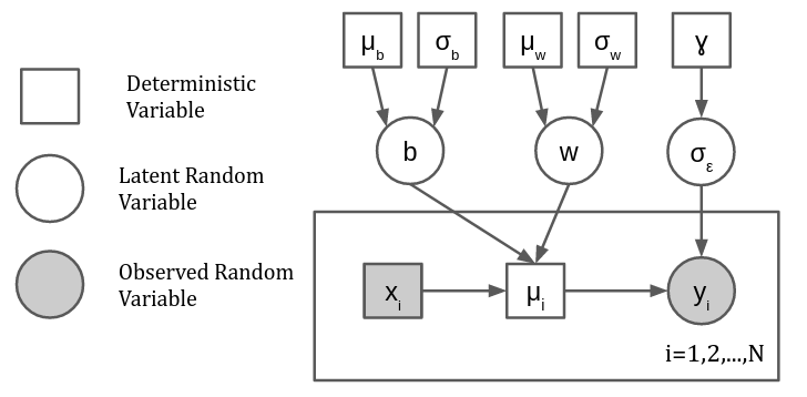
with hyperparameters \(\mu_b = \mu_\sigma=0\) and \(\sigma_b = \sigma_w = \gamma = 10\)
def model(x, y=None):
    w = numpyro.sample("w", dists.Normal(0.0, 10.0))
    b = numpyro.sample("b", dists.Normal(0.0, 10.0))
    s = numpyro.sample("s_eps", dists.HalfCauchy(10.0))
    with numpyro.plate("data", size=len(x)):
        mu = numpyro.deterministic("mu", x*w+b)
        y = numpyro.sample("y", dists.Normal(mu, s), obs=y)
    return mu
In what follows we review how to set-up the SVI object to obtain a variational posterior for this numpyro model
Guide function
The guide represents \(q_\nu(\theta)\), i.e. it has to specify the approximate posterior distribution of the parameters of the model
In practice, a numpyro guide is a Python function that has to comply with the following:
The input arguments have to be the same as those in the model function
Every
numpyro.samplein the model function needs anumpyro.sampleusing the same name in the guideThe primitive
numpyro.paramis used to register the hyperparameters of these latent variables
For the bayesian linear regression \(\theta = (w, b, s)\). As an example we will implement a fully factored normal guide following
The hyperparameters are \(\nu = (\mu_w, \sigma_w, \mu_b, \sigma_b, \mu_{\log s}, \sigma_{\log s})\). We need to register every parameter in \(\nu\) using numpyro.param as these are the values that we will optimize using SVI
from numpyro.distributions import constraints

def guide(x, y=None):
    # slope
    w_loc = numpyro.param("w_loc", 0.0)
    w_scale = numpyro.param("w_scale", 0.1, constraint=constraints.positive)
    w = numpyro.sample("w", dists.Normal(w_loc, w_scale))
    # intercept
    b_loc = numpyro.param("b_loc", 0.0)
    b_scale = numpyro.param("b_scale", 0.1, constraint=constraints.positive)
    b = numpyro.sample("b", dists.Normal(b_loc, b_scale))
    # noise variance
    s_loc = numpyro.param("s_log_loc", 0.0)
    s_scale = numpyro.param("s_log_scale", 0.1, constraint=constraints.positive)
    s = numpyro.sample("s_eps", dists.TransformedDistribution(dists.Normal(s_loc, s_scale),
                                                          dists.transforms.ExpTransform()))
Note
We can restrict the value taken by a param using the constraint argument. The constraints submodule offers non-negativity, truncated, circular and simplex constraints, among others
Loss function
In the previous lesson we studied the Evidence Lower Bound (ELBO)
where
The model function defines \(p(\mathcal{D}|\theta) p (\theta)\)
The guide function defines \(q_\nu(\theta)\)
Numpyro offers several versions of the ELBO in numpyro.infer, the most common are:
Trace_ELBO: Default ELBO. Reduces variance of the gradients using “Rao-Blackwellization”TraceMeanField_ELBO: Assumes Mean-field structure. Reduce variance of gradients using analytical KL when possible
We will study the importance of gradient variance later
Training
The main methods of the SVI object are
init: Expects a PRNG key and the model/guide arguments. Initializes the SVI object and returns an SVI stateget_params: Expects an SVI state. Returns a dictionary with the model parametersupdate: Expects an SVI state and the model/guide arguments. Performs a gradient descent step. Returns the update state and the value of the loss
Note
svi.update is similar to the backward() plus step() in pytorch
In this example we select the Adam algorithm as optimizer and the default ELBO as loss function. The example also demostrates how to use jax.jit to improve the computational efficiency of update
Note
Any optax optimizer can be used with SVI
%%time

from jax import jit
import optax
from tqdm.notebook import tqdm

def train_svi(guide, key, lr=0.01, nepochs=1000):
    svi = numpyro.infer.SVI(model, guide, optax.adam(lr), loss=numpyro.infer.Trace_ELBO())
    state = svi.init(key, x, y)

    loss_evolution = []
    param_names = list(svi.get_params(state).keys())
    print(param_names)
    param_evolution = {param: [] for param in param_names}

    jit_update = jit(svi.update)
    for epoch in tqdm(range(nepochs)):
        state, loss = jit_update(state, x, y)
        loss_evolution.append(loss.item())
        current_params = svi.get_params(state)
        for name, value in current_params.items():
            param_evolution[name].append(value)

    for name, value in current_params.items():
        param_evolution[name] = jnp.stack(param_evolution[name])
    return svi, state, loss_evolution, param_evolution

key, key_ = random.split(key)
svi, state, loss_evolution, param_evolution = train_svi(guide, key_)
['b_loc', 'b_scale', 's_log_loc', 's_log_scale', 'w_loc', 'w_scale']
CPU times: user 4.59 s, sys: 30 ms, total: 4.62 s
Wall time: 4.62 s
The evolution of the ELBO:
hv.Curve(loss_evolution, 'Epoch', 'Loss').opts(width=500)
And the evolution of the registered parameters:
curves = [hv.Curve(param_evolution[name],
                   'Epoch', 'Locations', label=name) for name in ['b_loc', 'w_loc', 's_log_loc']]
loc_plots = hv.Overlay(curves).opts(legend_position='top', width=320)
curves = [hv.Curve(param_evolution[name],
                   'Epoch', 'Scales', label=name) for name in ['b_scale', 'w_scale', 's_log_scale']]
scale_plots = hv.Overlay(curves).opts(legend_position='top', width=320)
loc_plots + scale_plots
Tip
When learning more complex models on larger datasets we should consider partitioning the dataset into training and validation subsets to verify ELBO convergence (early stopping).
Inspecting the posterior
The Predictive object from numpyro.infer can be used to obtain the posterior of the parameters and the predictive posterior over new test data
Instead of passing posterior_samples (as in MCMC) we pass the guide function and the learned parameters
predictive = numpyro.infer.Predictive(model,
                                      guide=svi.guide,
                                      params=svi.get_params(state),
                                      return_sites=['w', 'b', 's_eps', 'mu'],
                                      num_samples=1000)

x_test = jnp.linspace(-12, 12, num=100)
posterior_samples = predictive(random.PRNGKey(1), x_test)
def plot_marginals(posterior_samples):
    dist_w = hv.Distribution(posterior_samples['w'], 'w') * hv.VLine(w_true)
    dist_b = hv.Distribution(posterior_samples['b'], 'b') * hv.VLine(b_true)
    dist_s = hv.Distribution(posterior_samples['s_eps'], 's_eps') * hv.VLine(s_true)
    return dist_b + dist_w + dist_s

plot_marginals(posterior_samples)
def plot_joint_posterior(posterior_samples, param1, param2):
    posterior = hv.Bivariate(jnp.stack((posterior_samples[param1], posterior_samples[param2])).T,
                             kdims=[param1, param2])
    return posterior.opts(cmap='Blues', line_width=0,
                          filled=True, width=300, axiswise=True)

hv.Layout([plot_joint_posterior(posterior_samples, 'w', 'b'),
           plot_joint_posterior(posterior_samples, 's_eps', 'b'),
           plot_joint_posterior(posterior_samples, 's_eps', 'w')
          ])
Note
Remember we used a factored normal guide, we expect no correlations
def plot_predictive(posterior_samples):
    low, mid, upper = jnp.quantile(posterior_samples['mu'], jnp.array([0.01, 0.5, 0.99]), axis=0)
    median = hv.Curve((x_test, mid)).opts(width=500, color='#30a2da')
    data = hv.ErrorBars((x, y, s_true))
    uncertainty = hv.Area((x_test, low, upper), vdims=['y', 'y2']).opts(color='#30a2da', alpha=0.3)
    return median * data * uncertainty

plot_predictive(posterior_samples)
Autoguides
Given a model, numpyro offers functions to generate guides automatically from it. These are found at numpyro.infer.autoguide
Note
The guide we previously wrote is roughly equivalent to AutoDiagonalNormal/AutoNormal, a guide where the latent variables are normal and independent
Other interesting auto guides are
AutoMultivariateNormal: Models correlation between the latent variablesAutoLowRankMultivariateNormal: Similar to the previous one, but using a low rank covariance matrix. Consider it when latent dimensionality is largeAutoDelta: Returns the Maximum a Posteriori estimateAutoLaplaceApproximation: Multivariate normal guide centered on the MAP with variance equal to the negative hessianAutoIAFNormal: Uses a sequence of bijective transformations starting from a Gaussian to obtain a more flexible distribution (more in this in future lessons)
The arguments of an AutoGuide are
A numpyro model
prefix(Optional): A string to name the internal parametersinit_loc_fn(Optional): An initialization scheme
Let’s see some examples
from numpyro.infer.autoguide import AutoDelta, AutoMultivariateNormal
%%time
key, key_ = random.split(key)
svi, state, loss_evolution, param_evolution = train_svi(AutoDelta(model, prefix='MAP'),
                                                        key_, nepochs=300)
['b_MAP_loc', 's_eps_MAP_loc', 'w_MAP_loc']
CPU times: user 3.49 s, sys: 13.3 ms, total: 3.5 s
Wall time: 3.51 s
hv.Curve(loss_evolution, 'Epoch', 'Loss').opts(width=500, logy=True)
svi.get_params(state)
{'b_MAP_loc': DeviceArray(-0.7979058, dtype=float32),
 's_eps_MAP_loc': DeviceArray(0.7400651, dtype=float32),
 'w_MAP_loc': DeviceArray(0.52685213, dtype=float32)}
predictive = numpyro.infer.Predictive(model,
                                      guide=svi.guide,
                                      params=svi.get_params(state),
                                      return_sites=['w', 'b', 's_eps', 'mu'],
                                      num_samples=1000)

x_test = jnp.linspace(-12, 12, num=100)
posterior_samples = predictive(random.PRNGKey(1), x_test)

plot_predictive(posterior_samples)
Note
The AutoDelta guide returns point estimates (MAP)
%%time
key, key_ = random.split(key)
svi, state, loss_evolution, param_evolution = train_svi(AutoMultivariateNormal(model, prefix='MVN'),
                                                        key_, nepochs=4000)
['MVN_loc', 'MVN_scale_tril']
CPU times: user 29.5 s, sys: 180 ms, total: 29.7 s
Wall time: 29.6 s
hv.Curve(loss_evolution, 'Epoch', 'Loss').opts(width=500, logy=True)
predictive = numpyro.infer.Predictive(model,
                                      guide=svi.guide,
                                      params=svi.get_params(state),
                                      return_sites=['w', 'b', 's_eps', 'mu'],
                                      num_samples=1000)

x_test = jnp.linspace(-12, 12, num=100)
posterior_samples = predictive(random.PRNGKey(1), x_test)

plot_marginals(posterior_samples)
hv.Layout([plot_joint_posterior(posterior_samples, 'w', 'b'),
           plot_joint_posterior(posterior_samples, 's_eps', 'b'),
           plot_joint_posterior(posterior_samples, 's_eps', 'w')
          ])
Note
The AutoMultivariateNormal guide models the correlation between \(b\) and \(w\)
plot_predictive(posterior_samples)
See also
See pyro’s tips and tricks for SVI, they apply to numpyro