NumPyro Basics¶

NumPyro is a probabilistic programming library that provides

Implementations of distributions, constraints and transforms
Primitives to specify elements in probabilistic models
Sampling (e.g. MCMC) and Optimization (e.g. VI) based inference algorithms

Numpyro uses jax as its backend for autograd and just-in-time (JIT) compilation to high performance hardware (GPUs/TPUs). NumPyro is very efficient but also lightweight and simple to use

Distributions¶

Several distributions are implemented in the numpyro.distributions submodule

As an example let’s create a normal distribution. This requires specifying its mean though loc and its standard deviation through scale

z = dists.Normal(loc=0.0, scale=1.0)
z

<numpyro.distributions.continuous.Normal at 0x7f35d31b0370>

We can then retrieve the values of the parameters using

z.loc, z.scale

(0.0, 1.0)

PDF and CDF

Distribution objects have a method called log_prob to compute the logarithm of the probability density function

x = jnp.linspace(-5, 5, num=100)
log_pdf = z.log_prob(x)

hv.Curve((x, jnp.exp(log_pdf))).opts(width=500)

There is also the cdf method to compute the cumulative density function

cdf_x = z.cdf(x)

hv.Curve((x, cdf_x)).opts(width=500)

Sampling

To get random samples from a distribution we use the sample o rsample methods. The latter uses reparametrization to sample, for example in this case of the gaussian

\[ z \sim N(\mu, \sigma^2) \]

is equivalent to the following reparametrization

\[\begin{split} \begin{split} \epsilon &\sim N(0, 1) \\ z &= \mu + \sigma \epsilon \end{split} \end{split}\]

This has several advantages that will be discussed in future lessons

Note

Not all distributions have rsample. The has_rsample attribute can be used to check if rsample is available

z.has_rsample

True

The sample and resample methods expects

pseudo random number generator key from jax.random
the shape of the sampled tensor: sample_shape

We can use the latter to sample a matrix of normal samples from a scalar normal distribution

key = random.PRNGKey(1234)
z.rsample(key, sample_shape=(3, 3))

DeviceArray([[ 1.3284667 ,  0.22779723, -0.5049753 ],
             [ 1.3871989 , -0.7382383 , -0.56204265],
             [ 0.5238776 ,  0.29912323, -0.01665386]], dtype=float32)

Shape

We can obtain the dimensions of the distribution using the shape method

z.shape()

()

In this example it is an empty tuple because we created a scalar distribution

Consider the following normal distribution with vector parameters

z = dists.Normal(loc=jnp.array([0, 10]), scale=jnp.array([1, 1]))
z

<numpyro.distributions.continuous.Normal at 0x7f35d0728f10>

The shape in this case is

z.shape()

(2,)

Note

This corresponds to two independent Normal distributions, that can be sampled together for convenience

key = random.PRNGKey(1234)
z.rsample(key, sample_shape=(5, ))

DeviceArray([[ 1.3284667 , 10.2277975 ],
             [-0.5049753 , 11.387199  ],
             [ 0.56284374,  9.437958  ],
             [ 0.5238776 , 10.299123  ],
             [-0.01665386, 10.882737  ]], dtype=float32)

Primitives for probabilistic graphical models¶

Consider the following probabilistic model

\[\begin{split} \begin{split} \mu &\sim \mathcal{N}(\mu_0, \sigma_0^2) \\ \sigma &\sim \log\mathcal{N}(\mu, \sigma_0^2) \\ x_i &\sim \mathcal{N}(\mu, \sigma^2) \\ \forall i &=1,\ldots,N \end{split} \end{split}\]

This model can be represented using a graph as

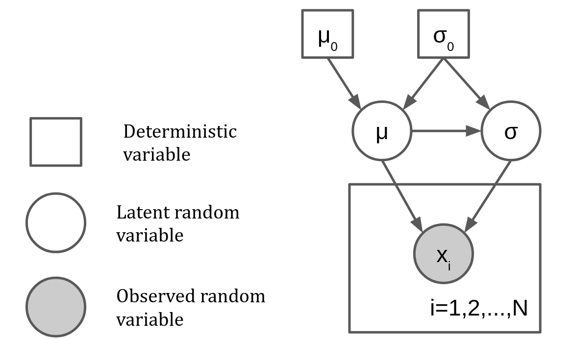
A probabilistic graphical model (PGM) is a statistical models were the relationships between variables (conditional dependence) are expressed through a graph. The key elements in PGMs are

Random variable (circle)
- Latent: We don’t have samples from it
- Observed: Wa have samples from it
Deterministic variable (square):
- Hyperparameters with a fixed value
- Result of deterministic function applied to random variables
Plate: Marks a group of variables that are conditionally independent given other variables

A PGM in NumPyro is a Python function that uses special primitives to represent these elements

Random Variables: numpyro.sample
Deterministic variables: numpyro.deterministic
Optimizable deterministic variable: numpyro.param
Plates: numpyro.plate

In NumPyro jargon these are refered to as sites. Numpyro keeps track of all sites when inference algorithms are run with the model

The model mentioned before written with NumPyro primitives would be:

mu0, s0 = 0., 1.

def model(x=None):
    mu = numpyro.sample(name='mu', fn=dists.Normal(loc=mu0, scale=s0))
    s = numpyro.sample(name='s', fn=dists.LogNormal(loc=mu, scale=s0))
    with numpyro.plate('data', size=len(x)):
        numpyro.sample(name='x', fn=dists.Normal(loc=mu, scale=s), obs=x)
    return mu, s # Return statement is optional

The sample primitive expects at least a unique name (name) and a distribution (fn). We can also supply data using the obs argument to create an observed random variable. Otherwise we are creating a latent random variable
The plate primitive is used as a context and expects a unique name and a size. If the data is multidimensional dim can be used to set the axis of conditional indepedence

Note

Within a plate context manager, sample sites will be automatically broadcasted to the size of the plate

We will use the following synthetic data to learn our model

Warning

If we were to run model we would get an AssertionError. To sample from the model we have to specify a pseudo random seed

We can pass a seed to our model using the seed handler

x = dists.Normal(0., 5.).rsample(sample_shape=(20,), key=random.PRNGKey(0))

for seed in range(5):
    with numpyro.handlers.seed(rng_seed=seed):
        print(model(x))

(DeviceArray(-1.2515389, dtype=float32), DeviceArray(0.15910524, dtype=float32))
(DeviceArray(-1.1470195, dtype=float32), DeviceArray(0.10654547, dtype=float32))
(DeviceArray(-0.16715223, dtype=float32), DeviceArray(1.1439366, dtype=float32))
(DeviceArray(-0.05887505, dtype=float32), DeviceArray(2.5868776, dtype=float32))
(DeviceArray(0.78741604, dtype=float32), DeviceArray(1.2294954, dtype=float32))

Sampling based Inference: MCMC¶

With the model set we move on inferring the posterior of its parameters and predictions

First we will review Markov Chain Monte Carlo (MCMC) to perform sampling based inference. MCMC methods return samples from a markov chain that converges to the posterior we care. We will focus on the practical implementation of MCMC using numpyro.

See also

For more deep theoretical details on MCMC see Barber Chapter 27 or here

The main wrapper for MCMC methods in numpyro is

numpyro.infer.MCMC(sampler,  # A sampler algoritm that decides the transitions
                   num_warmup, # Samples to discard in the beginning
                   num_samples, # Number of samples excluding the warmup ones
                   num_chains=1, 
                   thinning=1, # Fraction of post-warmup samples retained
                   ...
                   )

The main methods of MCMC are

run(): Populates the chain, expects the a PRNG key, the arguments of the model and initial values for the parameters
get_sample(): Returns the posterior samples
print_summary(): Returns a table with the statistics of the model parameters

Some of the samplers currently available are

Hamiltonian Monte Carlo: HMC
Hamiltonian Monte Carlo for mixed discrete and continuous variables: MixedHMC
Gradient-based Metropolis-Hastings: BarkerMH
No-U turn: NUTS

NUTS is a Hamiltonian methods that sets its step size automatically and is currently the state of the art. All kernels expects the function that specifies generative model plus their own particular arguments

%%time
from numpyro.infer import MCMC, NUTS

sampler = MCMC(sampler=NUTS(model, adapt_step_size=True), 
               num_chains=2, num_samples=1000, num_warmup=100, jit_model_args=True)

sampler.run(random.PRNGKey(1234), x)

/home/phuijse/.conda/envs/info320/lib/python3.10/site-packages/jax/_src/tree_util.py:185: FutureWarning: jax.tree_util.tree_multimap() is deprecated. Please use jax.tree_util.tree_map() instead as a drop-in replacement.
  warnings.warn('jax.tree_util.tree_multimap() is deprecated. Please use jax.tree_util.tree_map() '

CPU times: user 9.71 s, sys: 43.2 ms, total: 9.75 s
Wall time: 9.81 s

Plot the statistical moments, \(\hat r\) statistic and 90% credibility interval

sampler.print_summary(prob=0.9)

                mean       std    median      5.0%     95.0%     n_eff     r_hat
        mu      0.98      0.61      0.97     -0.05      1.96   1698.90      1.00
         s      6.02      0.98      5.88      4.60      7.53   1299.18      1.00

Number of divergences: 0

Get the samples and visualize the traces and posterior

samples = sampler.get_samples(group_by_chain=True)

def plot_trace(trace):
    names = list(trace.keys())
    plots = []
    for name in names:
        plot_param = []
        for i, chain in enumerate(samples[name]):
            plot_param.append(hv.Curve((chain), vdims=name, label=f'Chain {i}'))
        plots.append(hv.Overlay(plot_param))
    return hv.Layout(plots).cols(1).opts(hv.opts.Curve(width=600, height=150))
                            
plot_trace(samples)

samples = sampler.get_samples(group_by_chain=False)
names = list(samples.keys())
joint = jnp.stack(list(samples.values())).T

distb = hv.Distribution(joint[:, 0], names[0]).opts(height=125) * hv.VLine(0.0) * hv.VLine(float(x.mean()))
distw = hv.Distribution(joint[:, 1], names[1]).opts(width=125) * hv.VLine(5.0) * hv.VLine(float(x.std())) 
hv.Bivariate(joint, kdims=names).opts(cmap='Blues', line_width=0, filled=True, width=350) << distw << distb

Blue lines mark the true values used to generate the synthetic data
Red lines mark the MLE solutions

Bayesian Learning and Neural Networks

NumPyro Basics

Contents

NumPyro Basics¶

Distributions¶

Primitives for probabilistic graphical models¶

Sampling based Inference: MCMC¶