Non-linear LVMs: AutoEncoders¶

An autoencoder is an artificial neural networks for representation learning and dimensionality reduction

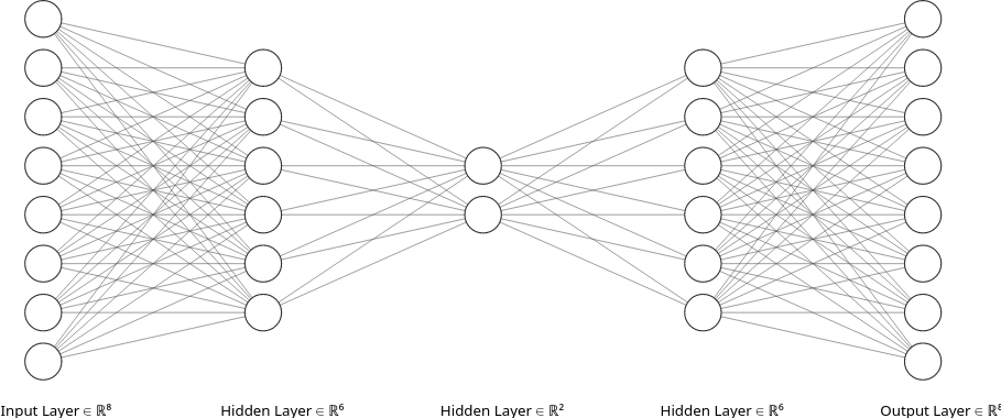
The following schematic exemplifies the architecture of an autoencoder

In general

The input and output dimensionality are equivalent
The code or bottleneck has a smaller dimensionality than the input/output

We call encoder to the neural network that maps the input to the code

\[ z = g_\phi(x) \]

and decoder to the neural network that maps the code to the output

\[ \hat x = f_\theta(z) \]

Autoencoders are trained by minimizing an error, e.g. the mean square error (MSE) or cross-entropy, between the input and the output

Note

In autoencoders the data is used as target (self-supervision)

For example we may use the MSE

\[ \hat \theta, \hat \phi = \text{arg} \min_{\phi, \theta} \| x - f_\theta(g_\phi(x)) \|^2 \]

which is equivalent to the maximum likelihood (MLE) solution assuming a spherical Gaussian likelihood (cross entropy is equivalent to the MLE given a Bernoulli likelihood)

Adding an L2 regularizer on \(\theta\) and \(\phi\) is equivalent to incorporating a spherical gaussian prior (MAP solution)

import holoviews as hv
hv.extension('bokeh')
hv.opts.defaults(hv.opts.Image(cmap='gray', xaxis=None, yaxis=None),
                 hv.opts.ErrorBars(lower_head=None, upper_head=None))

Example: In the following example we implement an autoencoder using fully connected (Dense) layers

There are several ways to achieve this in flax. In this case the encoder and decoder networks are implemented as separate flax modules for more flexibility

The Autoencoder class receives the previous two as arguments

from typing import Sequence, Callable
import flax.linen as nn

class Encoder(nn.Module):
    latent_dim: int
    hidden_units: Sequence[int]
    activation: Callable = nn.relu
        
    @nn.compact
    def __call__(self, x):
        for neurons in self.hidden_units:
            x = self.activation(nn.Dense(neurons)(x))
        return nn.Dense(self.latent_dim)(x)
    
class Decoder(nn.Module):
    output_dim: int
    hidden_units: Sequence[int]
    activation: Callable = nn.relu
        
    @nn.compact
    def __call__(self, x):
        for neurons in self.hidden_units:
            x = self.activation(nn.Dense(neurons)(x))
        return nn.Dense(self.output_dim)(x)    
        
class Autoencoder(nn.Module):
    encoder: nn.Module
    decoder: nn.Module
    
    @nn.compact
    def __call__(self, x):
        return self.decoder(self.encoder(x))

Note

No activation function is used for the final layers of the encoder and decoder networks. These layers corresponds to the latent projection and the reconstruction of the observed data, respectively.

In what follows the autoencoder is trained to reduce the dimensionality of the MNIST dataset

flax does not have built-in dataloaders as Pytorch. To shuffle the training dataset and deliver minibatches of data to the model we use this jax-based generator function:

import os
import sys
sys.path.append(os.path.abspath(os.path.join('../utils')))

from flax_dataloader import data_loader

import inspect
print(inspect.getsource(data_loader))

def data_loader(rng, x, y, batch_size, shuffle=False):
    steps_per_epoch = len(x) // batch_size

    if shuffle:
        batch_idx = random.permutation(rng, len(x))
    else:
        batch_idx = jnp.arange(len(x))

    batch_idx = batch_idx[: steps_per_epoch * batch_size]  # Skip incomplete batch.
    batch_idx = batch_idx.reshape((steps_per_epoch, batch_size))

    for idx in batch_idx:
        yield x[idx], y[idx] 

from mnist import mnist
train_images, train_labels, test_images, test_labels = mnist()

Each minibatch of images is processed using a rather generic train_step function. This function

Obtains the prediction (reconstruction) of the model
Computes the loss between prediction and labels
Computes the gradient of the loss
Updates the parameters

The jit decorator on top of the function triggers compilation the first time it is run. Subsequent calls will enjoy faster execution

import jax
import optax

@jax.jit
def train_step(state, batch):
    def loss_fn(params):
        logits = state.apply_fn({'params': params}, batch)
        return optax.sigmoid_binary_cross_entropy(logits, batch).mean()
    
    grad_fn = jax.value_and_grad(loss_fn)
    loss, grads = grad_fn(state.params)
    return loss, state.apply_gradients(grads=grads)

Note

MNIST are grayscale images with floating-point pixel values in the [0,1] range

Note

The output of the decoder is interpreted as the logits of the reconstructed images. Using the sigmoid_binary_cross_entropy as loss is the same as asumming a Bernoulli likelihood

To facilitate training, the TrainState from flax.training is used. This object carries the parameters, the state of the optimizer and the apply function of the model

import jax.random as random
import jax.numpy as jnp
from flax.training import train_state
from tqdm.notebook import tqdm

nepochs = 100
batch_size = 128
key = random.PRNGKey(12345)
model = Autoencoder(encoder=Encoder(hidden_units=[128, 128], latent_dim=2),
                    decoder=Decoder(hidden_units=[128, 128], output_dim=28*28))
dummy_batch = jnp.ones(shape=(batch_size, 28*28))
state = train_state.TrainState.create(apply_fn=model.apply, 
                                      params=model.init(key, dummy_batch)['params'],
                                      tx=optax.adamw(learning_rate=1e-3))

loss = []
for epoch in tqdm(range(nepochs)):
    key, key_ = random.split(key)
    train_loader = data_loader(key_, train_images, train_labels, batch_size, shuffle=True)
    minibatch_loss = []
    for batch, labels in train_loader:
        loss_val, state = train_step(state, batch)
        minibatch_loss.append(loss_val.item())
    loss.append(jnp.array(minibatch_loss).mean())
    
hv.Curve((range(nepochs), loss), 'Epoch', 'Loss').opts(width=500, height=200)

WARNING:absl:No GPU/TPU found, falling back to CPU. (Set TF_CPP_MIN_LOG_LEVEL=0 and rerun for more info.)

To obtain the test-set images projected to latent space we call the apply function of the encoder:

z = model.encoder.apply({'params': state.params["encoder"]}, test_images)

A scatter plot of the projections. Use the right-hand tools to zoom in and inspect it.

scatter_plot = []
for digit in range(10):
    mask = test_labels.argmax(axis=1) == digit
    scatter_plot.append(hv.Scatter((z[mask, 0], z[mask, 1]), 'z0', 'z1', label=f"{digit}"))
    
hv.Overlay(scatter_plot).opts(width=550, height=400, legend_position='right')

The following compare test set images with their reconstructions

Note

A sigmoid function is used to transform logits to equivalent pixel values

import numpy as np
xhat = nn.sigmoid(model.apply({'params': state.params}, test_images[:5]))

examples = [hv.Image(example.reshape(28, 28)) for example in test_images[:5]]
reconstructed = [hv.Image(example.reshape(28, 28)) for example in np.array(xhat[:5])]

hv.Layout(examples + reconstructed).opts(hv.opts.Image(width=100, height=100)).cols(5)

Reconstructions are much clearer than with the Linear LVM

Bayesian Learning and Neural Networks

Non-linear LVMs: AutoEncoders

Non-linear LVMs: AutoEncoders¶