Approximate Inference¶

For many interesting models (e.g. neural networks) the evidence

\[ p(\mathcal{D}|\mathcal{M}_i) = \int p(\mathcal{D}|\mathcal{M}_i, \theta) p(\theta| \mathcal{M}_i) d\theta \]

is intractable, i.e either the integral has no closed-form or the dimensionality is so big that numerical integration is not feasible

If the evidence is intractable then the posterior is also intractable

In these cases we resort to approximations

Stochastic approximation: For example Markov Chain Monte Carlo (MCMC). MCMC is computationally demanding (for complex models) but produces asymptotically exact samples from the intractable distribution
Deterministic approximation: For example Variational Inference (VI). VI is more efficient than MCMC, but it is not asymptotically exact. Instead of samples we get a direct approximation of the intractable distribution

The main topic of this lecture is deterministic approximations

The Laplace Approximation¶

In Bayesian statistics, the Laplace approximation refers to the application of Laplace’s method to approximate an intractable integral (evidence) using a Gaussian distribution

In particular, Laplace’s method is a technique to solve integrals of the form

\[ f(x) = \int e^{g(\theta)} d\theta, \]

by defining the auxiliary function as

\[\begin{split} \begin{split} g(\theta) &= \log p(\mathcal{D}| \theta) p(\theta) \\ &= \log p(\mathcal{D}| \theta) + \log p(\theta) \\ &= \sum_{i=1}^N \log p(x_i |\theta) + \log p(\theta) \end{split} \end{split}\]

then \(f(x)\) is equivalent to the evidence.

The “approximation” consists of performing a second order Taylor expansion of \(g(\theta)\) around \(\theta= \hat \theta_{\text{map}}\), i.e. the MAP solution. The result of this is

\[ g(\theta) \approx g(\hat \theta_{\text{map}}) - \frac{1}{2} (\theta - \hat \theta_{\text{map}})^T \Lambda (\theta - \hat \theta_{\text{map}}) \]

where

\[ \Lambda = -\frac{d^2 g}{d\theta^2} (\hat \theta_{\text{map}}), \]

is the negative Hessian evaluated at \(\hat \theta_{\text{map}}\)

Note

By definition the first derivative of \(g(\theta)\) evaluated at \(\hat \theta_{\text{map}}\) is zero

If we plug the Gaussian approximation back into the evidence we can now solve the integral as

\[\begin{split} \begin{split} p(\mathcal{D}) &\approx e^{g(\hat \theta_{\text{map}})} \int e^{-\frac{1}{2} (\theta - \hat \theta_{\text{map}})^T \Lambda (\theta - \hat \theta_{\text{map}})} d\theta \\ &= e^{g(\hat \theta_{\text{map}})} (2\pi)^{K/2} |\Lambda|^{-1/2} \end{split} \end{split}\]

where \(K\) is the dimensionality of \(\theta\). With this the posterior is

\[\begin{split} \begin{split} p(\theta| \mathcal{D}) &= \frac{p(\mathcal{D}|\theta) p(\theta) }{p(\mathcal{D})} = \frac{e^{ g(\theta)}}{\int e^{ g(\theta)} d\theta} = \\ &\approx \frac{1}{(2\pi)^{K/2} |\Lambda|^{-1/2}} e^{- \frac{1}{2} (\theta - \hat \theta_{\text{map}})^T \Lambda (\theta - \hat \theta_{\text{map}})} \end{split} \end{split}\]

Important

Laplace’s method approximates the posterior by a Multivariate Gaussian centered on the MAP.

Warning

As the following figure shows, Laplace’s method might not be the “best” gaussian fit to our distribution

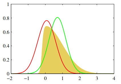
A non-gaussian distribution is shown in yellow. The red line corresponds to a gaussian centered on the mode (Laplace approximation), while the green line corresponds to a gaussian with minimum reverse KL divergence

Requirement of the Laplace approximation

For Laplace’s approximation the MAP solution and the negative Hessian evaluated at the MAP solution are needed

In the first place \(g(\theta)\) has to be continuous and differentiable on \(\theta\), and the negative Hessian has to be positive definite

A closer look to the evidence in Laplace approximation

Using Laplace approximation the log evidence can be decomposed as

\[\begin{split} \begin{split} \log p(\mathcal{D}|\mathcal{M}_i) &\approx g(\hat \theta_{\text{map}}) + \frac{K}{2} \log(2\pi) - \frac{1}{2} \log | \Lambda | \\ &=\log p(\mathcal{D}|\mathcal{M}_i, \hat \theta_{\text{map}}) + \log p(\hat \theta_{\text{map}}| \mathcal{M}_i) + \frac{K}{2} \log(2\pi) - \frac{1}{2} \log | \Lambda | \end{split} \end{split}\]

i.e. the log evidence is approximated by the best likelihood fit plus the Occam’s factor

The Occam’s factor depends on the

log pdf of \(\theta\): Prior
number of parameters \(K\): Complexity
second derivative around the MAP: Model uncertainty

Relationship between the evidence in Laplace approximation and the BIC

In the regime of very large number of samples (\(N\)) it can be shown that Laplace’s approximations is dominated by

\[ \log p(\mathcal{D}|\mathcal{M}_i) \approx \log p(\mathcal{D}|\mathcal{M}_i, \hat \theta_{\text{mle}}) - \frac{K}{2} \log N, \]

where \(\theta_{\text{mle}}\) is the maximum likelihood solution.

The expression above is equivalent to the negative of the Bayesian Information Criterion (BIC)

Variational Inference¶

In this section we review a more general method for deterministic approximation. Remember that we are interested in the (intractable) posterior

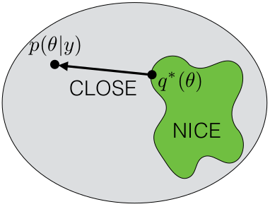
\[ p(\theta|\mathcal{D}) = \frac{p(\mathcal{D}|\theta) p(\theta)}{p(\mathcal{D})} \]

Variational Inference (VI) is a family of methods in which a simpler (tractable) posterior distribution is proposed to “replace” \(p(\theta|\mathcal{D})\). This simpler posterior is denoted as \(q_\nu(\theta)\) which represents a family of distributions parameterized by \(\nu\)

Optimization problem: The objective is to find \(\nu\) that makes \(q\) most similar to \(p\)

We can formalize this as a KL divergence minimization problem

\[ \hat \nu = \text{arg}\min_\nu D_{\text{KL}}[q_\nu(\theta) || p(\theta|\mathcal{D})] = \int q_\nu(\theta) \log \frac{q_\nu(\theta)}{p(\theta|\mathcal{D})} d\theta, \]

but this expression depends on the intractable posterior. To continue we use Bayes Theorem to move the evidence out from the integral

\[ D_{\text{KL}}[q_\nu(\theta) || p(\theta|\mathcal{D})] = \log p(\mathcal{D}) + \int q_\nu(\theta) \log \frac{q_\nu(\theta)}{p(\mathcal{D}, \theta)} d\theta \]

As \(p(\mathcal{D})\) does not depend on \(\nu\) we can focus on the right hand term. The optimization problem is typically written as

\[ \hat \nu = \text{arg}\max_\nu \mathcal{L}(\nu) =\int q_\nu(\theta) \log \frac{p(\mathcal{D}, \theta)}{q_\nu(\theta)}d\theta \]

where \( \mathcal{L}(\nu)\) is called the Evidence Lower BOund (ELBO).

The name comes from the fact that

\[ \log p(\mathcal{D}) \geq \mathcal{L}(\nu) = \int q_\nu(\theta) \log \frac{p(\mathcal{D}, \theta)}{q_\nu(\theta)}d\theta, \]

which is a result of the non-negativity of the KL divergence.

Ideally we choose a “simple-enough” parametric family \(q\) so that the ELBO is tractable

Note

The ELBO can only be tight if \(p\) is within the family of \(q\)

More attention on the ELBO¶

The ELBO can also be decomposed as

\[\begin{split} \begin{split} \mathcal{L}(\nu) &= \int q_\nu(\theta) \log \frac{p(\mathcal{D}|\theta) p (\theta)}{q_\nu(\theta)}d\theta \\ &= \int q_\nu(\theta) \log p(\mathcal{D}|\theta) d\theta - \int q_\nu(\theta) \log \frac{q_\nu(\theta)}{ p (\theta)} d\theta \\ &= \mathbb{E}_{\theta \sim q_\nu(\theta)} \left[\log p(\mathcal{D}|\theta)\right] - D_{KL}[q_\nu(\theta) || p(\theta)] \end{split} \end{split}\]

From which we can recognize that maximizing the ELBO is equivalent to:

Maximizing the log likelihood for parameters sampled from the approximate posterior: Generative model produces realistic data samples
Minimizing the KL divergence between the approximate posterior and prior: Regularization for the approximate posterior

Another way to “obtain” the ELBO

We can get the ELBO using Jensen’s inequality on the log evidence

\[\begin{split} \begin{split} \log p(\mathcal{D}) &= \log \mathbb{E}_{\theta\sim p(\theta)} \left[p(\mathcal{D}|\theta)\right]\nonumber \\ &= \log \mathbb{E}_{\theta\sim q_\nu(\theta)} \left[p(\mathcal{D}|\theta)\frac{p(\theta)}{q_\nu(\theta)}\right] \\ &\geq \mathbb{E}_{\theta\sim q_\nu(\theta)} \left[\log \frac{p(\mathcal{D},\theta)}{q_\nu(\theta)}\right] =\int q_\nu(\theta) \log \frac{p(\mathcal{D},\theta)}{q_\nu(\theta)}d\theta \end{split} \end{split}\]

A simple posterior: Fully-factorized posterior¶

A broadly-used idea to make posteriors tractable is to assume that there is no correlation between factors

\[ q_\nu(\theta) = \prod_{i=1}^K q_{\nu}(\theta_i), \]

this is known as the Mean-field VI

Replacing this factorized posterior on the ELBO

\[\begin{split} \begin{split} \mathcal{L}_\text{MF}(\nu) &= \int \prod_{i=1}^K q_{\nu}(\theta_i) \left ( \log p(\mathcal{D}, \theta) - \sum_{i=1}^K \log q_{\nu}(\theta_i) \right) d\theta \\ &= \int q_{\nu_i}(\theta_i) \left [ \int \prod_{j\neq i} q_{\nu_j}(\theta_j) \log p(\mathcal{D}, \theta) d\theta_j \right ] d\theta_i - \sum_{i=1}^K \int q_{\nu_i}(\theta_i) \log q_{\nu_i}(\theta_i) d\theta_i \\ \end{split} \end{split}\]

Asumming that we keep all \(\theta\) except \(\theta_i\) fixed, we can update \(\theta_i\) iteratively using

\[ \mathcal{L}_\text{MF}(\nu_i) = \int q_{\nu_i}(\theta_i) \mathbb{E}_{\prod q_{i\neq j}} \left[ \log p(\mathcal{D},\theta) \right ] d\theta_i - \int q_{\nu_i}(\theta_i) \log q_{\nu_i}(\theta_i) d\theta_i + \text{Constant} \]

Note

(In this case) Maximizing the ELBO is equivalent to minimizing the KL between \(q_{\nu_i}(\theta_i)\) and \(\mathbb{E}_{\prod q_{i\neq j}} \left[ p(\mathcal{D}, \theta) \right ]\)

The optimal \(q\) in this case is given by

\[ q_i(\nu_i) \propto \exp \left ( \mathbb{E}_{\prod q_{i\neq j}} \left[ p(\mathcal{D}, \theta) \right ] \right ) \]

Bayesian Learning and Neural Networks

Approximate Inference

Contents

Approximate Inference¶

The Laplace Approximation¶

Variational Inference¶

More attention on the ELBO¶

A simple posterior: Fully-factorized posterior¶